I walked through the grad student computer lab today, and heard one of my colleagues talking to herself: "I hate calculating final grades! It takes forever, and I'm always afraid I'm going to make a mistake and keep someone from graduating." It turned out that she was sifting through the gradebook by hand to drop low quiz scores and was manually entering final grades based on the point total.
The great news is - Microsoft Excel can automate these tasks, ensuring mistake-free final grades. Here's how:
Drop lowest score(s)
It's fairly common for instructors to allow students to drop the lowest score or two, especially on assignments like quizzes or short weekly writing exercises. This method will also work for assignments where students are only required to complete a subset of the available tasks (e.g., students must respond to at least 8 of the 10 weekly writing prompts).
Drop single score
To drop a single score in Excel, it is easiest if the columns containing the scores are adjacent to one another. The example below shows a gradebook containing scores for six quizzes in columns B through G.
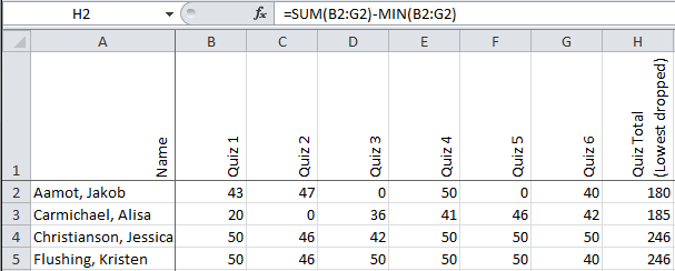
To drop the lowest score and add the remaining scores for hypothetical student Jakob Aamot, use the formula:
=SUM(B2:G2)-MIN(B2:G2)
In words, this formula adds up all of the scores in row 2 columns B through G, then subtracts the minimum (lowest) score in row 2 columns B through G. Once you have the formula in your Excel sheet, you can copy and paste it down through your total column for as many students as you have - Excel will intelligently change the row number in pasted formulas.
Drop multiple scores
To drop multiple scores, a slightly different formula must be used.
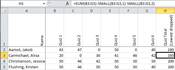
To drop the lowest two scores for hypothetical student Alisa Carmichael, use the formula:
=SUM(B3:G3)-SMALL(B3:G3,1)-SMALL(B3:G3,2)
In words, this formula is adds up all of the scores in row 3 columns B through G, then subtracts the first smallest score in row 3 columns B through G, then subtracts the second smallest score in row 3 columns B through G. The ",1" or ",2" after the cell range B3:G3 tells Excel to drop the first or second smallest score, respectively. If you wish to drop more than two scores, just add an additional "-SMALL(B3:G3,#" to the end of the formula, replacing "#" with the rank of the next highest score to drop.
Convert points or percentages to letter grades
Instead of going through the gradebook and manually entering letter grades based on point totals or class percentages, an Excel formula can automatically report the appropriate letter grade based on your grading scheme.

In this hypothetical example, the course percent earned determines the final grade according to a typical +/- grading scheme. The formula looks big and complicated, but it's really just the same formula repeated over and over with minor modifications. To calculate the final grade for Jakob Aamot, use the formula:
=IF(B2>=97,"A+",IF(B2>=93,"A",IF(B2>=90,"A-",IF(B2>=87,"B+",IF(B2>=83,"B",
IF(B2>=80,"B-",IF(B2>=77,"C+",IF(B2>=73,"C",IF(B2>=70,"C-",IF(B2>=67,"D+",
IF(B2>=63,"D",IF(B2>=60,"D-","F"))))))))))))
In words, this formula looks at the score in row 2 column B. If the number is larger than or equal to 97, it sets the value of row 2 column C to A+. If the number is not larger than or equal to 97, it continues down the formula path until the number in row 2 column B is larger than or equal to the listed value. If none of those numbers work, it sets the value of row 2 column C to F.
If using a point system rather than percentages, you can use the same formula, just replace the percentages with the appropriate cut-off point totals for each grade. Similarly, if your grading scale is different, just replace the current grade designations with your own.